User's Manual for ML-Relate

Citation

Kalinowski ST, AP Wagner, ML Taper (2006) ML-Relate: a computer program for maximum likelihood estimation of relatedness and relationship. Molecular Ecology Notes 6:576-579.

Quick Start

The normal order of operations for analyzing data is as follows.

1. Open GENEPOP data file.
2. Check summary statistics (sample size, number of alleles, etc.) to verify that data has been read correctly.
3. Perform Hardy-Weinberg test to detect null alleles.
4. If null alleles are present, specify which loci have nulls.
5. Estimate relatedness or relationship for pairs of individuals.

Introduction

ML-Relate is a Microsoft Windows based computer program that calculates maximum likelihood estimates of relatedness and relationship from codominant genetic data (e.g. microsatellites, allozymes, SNPs). The program was designed to accommodate microsatellite loci with null alleles. The purpose of this manual is two-fold: 1) to assist the user in running the program, and 2) to point the user to the primary literature where the calculations performed by ML-Relate are described in detail.

Program Requirements

ML-Relate should run on any Microsoft Windows operating system since Windows 98. It also requires the Microsoft .NET (pronounced "dot net") framework 1.1. The .NET Framework 1.1 is a component of the Microsoft Windows operating system used to build and run Windows-based applications. If you have a recent version of Windows, you probably already have .NET installed on your computer. You can check by clicking Start on your Windows desktop, selecting Control Panel, and then double-clicking the Add or Remove Programs icon. When that window appears, scroll through the list of applications. If you see Microsoft .NET Framework 1.1 listed, the latest version is already installed and you do not need to install it again.

If you do not have .NET already installed on your computer, you have two options for installing it:

1. Update your operating system. This is relatively painless. To begin, open Microsoft Explorer, select Tools > Windows Update, find Microsoft .NET framework 1.1 and install it (It will be listed under "Pick updates to install").
2. Download the Microsoft .NET Framework Version 1.1 Redistributable Package, and run the executable file "dotnetfx.exe." The easiest way to do this may be to follow the link posted at www.montana.edu/kalinowski/kalinowski_software.htm.

Installation

To "install," place ML-Relate.exe and kalinowski_library.dll in a folder. Click on ML-Relate.exe to run. Delete both files to "uninstall."

Input files

ML-Relate needs two types of data genotypes of the individuals to analyze, and allele frequencies for the population that the individuals belong to. This data is contained in a GENEPOP file (Raymond & Rousset 1995; http://wbiomed.curtin.edu.au/genepop/). An example is shown in Appendix 1. ML-Relate will read genotypes having either four or six characters per genotype.

GENEPOP files read by ML-Relate can be structured in two ways, depending on how the user wants to specify allele frequencies for the population. The simplest approach is to estimate allele frequencies from the individuals whose relatedness is being analyzed. In order to do this, place all of the genotypes in a single POP (to use the GENEPOP term). In other cases, users may wish to specify different allele frequencies for the population (which might be appropriate if genotypes are available for adults and offspring separately). In order to do this, make a GENEPOP file with two POPs. The first POP should have the genotypes for ML-Relate to estimate allele frequencies. The second POP should have the genotypes for the individuals to analyze.

Summary Statistics

ML-Relate will calculate the following summary statistics: sample size, number of alleles observed per locus, expected heterozygosity, and allele frequencies observed at each locus. These functions are useful for verifying that ML-Relate read an input file correctly.
Sample size. The sample size (in genes) for each locus.
Number of alleles. The number of alleles observed at each locus.
Observed allele frequencies. The frequency of each allele in the data file. These frequencies do not account for the potential presence of null alleles.

Expected heterozygosity. Neis (1978) unbiased estimate of expected heterozygosity.

Null alleles

ML-Relate can adjust relatedness/relationship calculations to accommodate null alleles (see Dakin & Avise 2004 for a review of null alleles). In order to do this, the user must specify which loci have null alleles. This is done with the Nulls>Specify which loci have null alleles menu. If the user does not already know which loci have nulls, ML-Relate provides a Hardy-Weinberg equilibrium test to detect a deficiency of heterozygosity. This test is available from the Nulls>Hardy-Weinberg test for heterozygote deficiency menu. The specific test used by ML-Relate is the Monte-Carlo randomization test of Guo & Thompson (1992) using the U-statistic of Rousset & Raymond (1995). The test is one-tailed, i.e. it estimates the probability of obtaining the observed U statistic or a greater value under Hardy-Weinberg conditions. When null alleles are present (as specified by the user), ML-Relate uses maximum likelihood estimates of the frequency of null alleles in all calculations. The method is described in detail by Kalinowski & Taper (2006). This method was chosen because it usually is more accurate than the estimators of Chakraborty et al. (1992), Brookfield (1996), Summers & Amos (1997). Estimates of allele frequencies at loci with null alleles can be viewed from the Nulls>Estimate allele frequencies with NULL allele PRESENT menu.

Estimating Relatedness

ML-Relate calculates maximum likelihood estimates of relatedness (r) (See Blouin 2003 for a review). This method was chosen because maximum likelihood estimates of relatedness usually are more accurate than other estimators (Milligan 2003). Likelihood calculations are described in detail by Wagner et al. (2006). ML-Relate uses the downhill simplex routine to find the maximum likelihood estimate of r. Experience (S. Kalinowski, unpublished) has shown that likelihood surfaces for r can have multiple peaks. Therefore, the downhill simplex routine is started from 11 sets of points, one of which is {Unrelated, Full Sibs, Parent/Offspring}. The other ten are random values.

The user has three options for estimating relatedness. If the List option is chosen, results are output in the form of a list. If the Matrix option is chosen, results are output in the form of a matrix. If the Two Specific Individuals option is chosen, ML-Relate will estimate r for one pair of individuals only.

Estimating Relationship

ML-Relate is useful for discriminating among four common pedigree relationships: unrelated (U), half-siblings(HS), full-siblings (FS), and parent-offspring (PO). The list below shows the options available in the Relationship menu. Each item in the menu is described in the sections that follow.

Relationships

> Estimate Relationship > Matrix Output
> Estimate Relationship > List Output
> Estimate Relationship > Two specific individuals
> Confidence Sets
> Specific hypothesis test

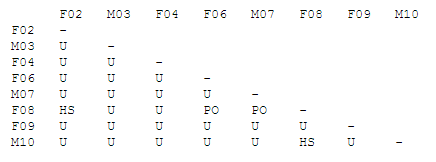
Estimate Relationship > Matrix Output

This function calculates the likelihood of four relationships (U, HS, FS, PO) for each pair of individuals are outputs a matrix of the relationships that have the highest likelihood for each pair of individuals. An example is shown below.

Estimate Relationship > List Output

This function lists the log-likelihood of four relationships (U, HS, FS, PO) for all pairs of individuals. The output requires some explanation. See the example below.

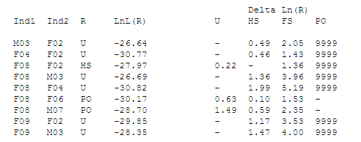
The two columns on the left, Ind1 and Ind 2, list the ID of pairs of individuals (e.g., M03 & FO2). The next column, R, lists the relationship with the highest likelihood. For example, this is U for individuals M03 and F02. The next column, LnL(R), lists the natural logarithm of R. The four remaining columns list the delta log-likelihoods for each relationship. These numbers represent differences on a log scale. Consider the first row. The value 0.49 shown below HS indicates that the likelihood of individuals M03 and F02 being HS is 0.49 less than the likelihood of the individuals being U (the maximum likelihood relationship). In other words, LnL(HS) = -26.64  0.49 = -27.13. If a relationship is excluded by genetic data, a relative LnL of 9999 is shown. For example, two individuals can be excluded as parent/offspring (PO) if they share no alleles.

Confidence Sets

This function produces a confidence set for the relationship between pairs of individuals. Example output is shown below.

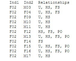
In this example, three relationships are consistent with the genotypes at individuals F02 and M03 (U, HS, FS). In contract, only one relationship is consistent with the genotypes at individuals F02 and F14 (FS). Simulation is used to perform these statistical tests (Kalinowski et al. 2006), and the user must specify how many random genotypes must be simulated for each test.

Specific hypothesis test

This function is best described with an example. Assume that a researcher observes two adult female hyenas in the proximity of a den and wants to determine whether the hyenas are siblings or unrelated. Genetic data is collected and ML-Relate indicates that the relationship full-siblings has the highest likelihood. However, the likelihood for unrelated is not much lower, and the researcher wonders if the hyenas are actually unrelated, but have genotypes that suggest a sibling relationship by chance. The statistical test performed by this function evaluates this possibility.

The following dialog box is used.

The putative relationship between two individuals is the relationship suspected by the researcher apriori. It is the relationship with the higher likelihood. The alternative relationship is the one this test tries to exclude. It is the relationship with the lower likelihood. Simulation is used to perform the test, and the user must specify how many random genotype pairs to simulate. If the p-value for the test is low, the user can reject the alternative hypothesis (See Kalinowski et al. 2006 for details).

History

1 Oct 2005 ML-Relate first posted on the internet.

Bugs

No bugs have been detected (yet?).

Literature Cited

• Blouin MS (2003) DNA-based methods for pedigree reconstruction and kinship analysis
• Dakin EE, Avise JC (2004). Microsatellite null alleles in parentage analysis. Heredity 93: 504-509.
• Guo SW, EA Thompson (1992) Performing the exact test of Hardy-Weinberg proportions for multiple alleles. Biometrics 48: 361-372.
• Kalinowski ST, ML Taper (2005) Maximum likelihood estimation of the frequency of null alleles at microsatellite loci. Conservation Genetics, (In review).
• Milligan BG (2003). Maximum-likelihood estimation of relatedness. Genetics 163: 1153-1167.
• Nei M (1978). Estimation of average heterozygosity and genetic distance from
• a small number of individuals. Genetics 89: 583-590.
• Press WH, SA Teukolsky, WT Vetterling, BP Flannery (1992) Numerical Recipes in C. The Art of Scientific Computing 2nd Ed. Cambridge University Press.
• Raymond M, F Rousset (1995) GENEPOP (version 1.2): Population genetics software for exact tests and ecumenicism. Journal of Heredity, 86, 248-249.
• Rousset F, M Raymond (1995) Testing heterozygote excess and deficiency. Genetics 140, 1413-1419.
• Wagner AP, S Creel, ST Kalinowski (2005) Estimating relatedness and relationships using microsatellite loci with null alleles. Heredity, (Accepted pending revision).

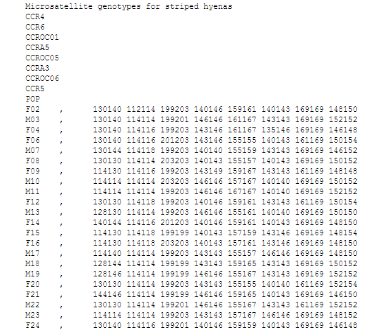
Appendix 1. Example of a GENEPOP data file. The file contains diploid genotypes for eight microsatellite loci (CCR4, CCR6, CCROC1, CCRA6, CCROC05, CCRA3, CCROC06, CCR5).

For example, the genotype of individual F02 at locus CCR6 is 112/114. Microsatellite genotypes for striped hyenas.